7-Main_NLP_tasks-2-Fine-tuning_a_masked_language_model

中英文对照学习，效果更佳！
原课程链接：https://huggingface.co/course/chapter7/3?fw=pt

Fine-tuning a masked language model

微调屏蔽语言模型

For many NLP applications involving Transformer models, you can simply take a pretrained model from the Hugging Face Hub and fine-tune it directly on your data for the task at hand. Provided that the corpus used for pretraining is not too different from the corpus used for fine-tuning, transfer learning will usually produce good results.

在Studio Lab的Colab Open中提出问题对于许多涉及Transformer模型的NLP应用程序，您只需从Hugging Face中心获取一个预先训练的模型，并直接根据您的数据对其进行微调，以完成手头的任务。只要用于预训练的语料库与用于微调的语料库差别不大，迁移学习通常会产生良好的效果。

However, there are a few cases where you’ll want to first fine-tune the language models on your data, before training a task-specific head. For example, if your dataset contains legal contracts or scientific articles, a vanilla Transformer model like BERT will typically treat the domain-specific words in your corpus as rare tokens, and the resulting performance may be less than satisfactory. By fine-tuning the language model on in-domain data you can boost the performance of many downstream tasks, which means you usually only have to do this step once!

然而，在少数情况下，在培训特定于任务的负责人之前，您需要首先微调数据的语言模型。例如，如果您的数据集包含法律合同或科学文章，像Bert这样的普通Transformer模型通常会将语料库中特定于领域的单词视为稀有标记，结果可能不太令人满意。通过对域内数据的语言模型进行微调，您可以提高许多下游任务的性能，这意味着您通常只需执行此步骤一次！

This process of fine-tuning a pretrained language model on in-domain data is usually called domain adaptation. It was popularized in 2018 by ULMFiT, which was one of the first neural architectures (based on LSTMs) to make transfer learning really work for NLP. An example of domain adaptation with ULMFiT is shown in the image below; in this section we’ll do something similar, but with a Transformer instead of an LSTM!

这种在领域内数据上微调预先训练的语言模型的过程通常被称为领域适应。它于2018年由ULMFiT推广，这是第一批(基于LSTM)使迁移学习真正适用于NLP的神经体系结构之一。下图显示了使用ULMFiT进行域适配的示例；在本节中，我们将执行类似的操作，但使用的是Transformer而不是LSTM！

By the end of this section you’ll have a masked language model on the Hub that can autocomplete sentences as shown below:

ULMFiT。ULMFiT。在本小节结束时，您将在Hub上拥有一个可以自动补全句子的屏蔽语言模型，如下所示：

Let’s dive in!

让我们跳下去吧！

🙋 If the terms “masked language modeling” and “pretrained model” sound unfamiliar to you, go check out [Chapter 1], where we explain all these core concepts, complete with videos!

🙋如果您对“掩蔽语言建模”和“预先训练的模型”这两个术语听起来不熟悉，请查看第1章，我们将在其中解释所有这些核心概念，并提供视频！

Picking a pretrained model for masked language modeling

为掩蔽语言建模选择一个预先训练的模型

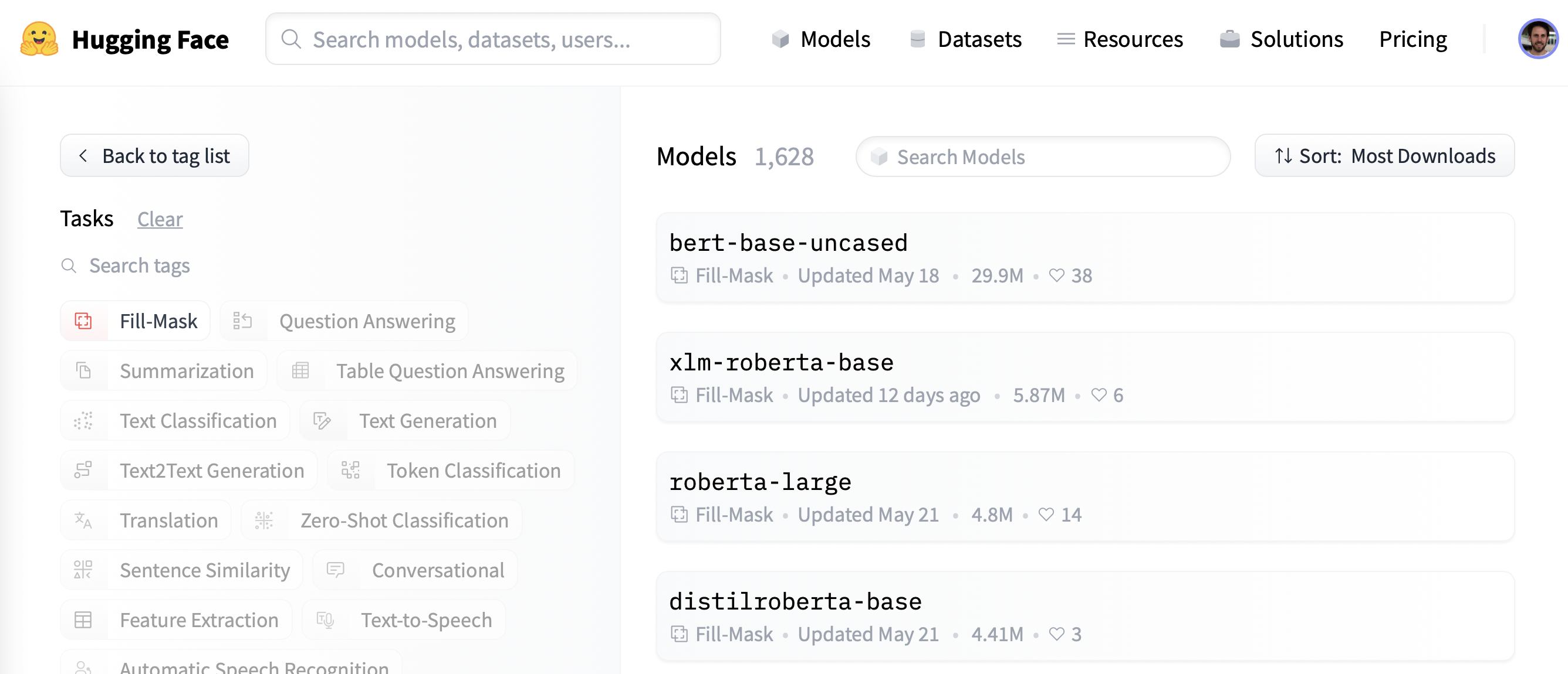
To get started, let’s pick a suitable pretrained model for masked language modeling. As shown in the following screenshot, you can find a list of candidates by applying the “Fill-Mask” filter on the Hugging Face Hub:

首先，让我们为掩蔽语言建模选择一个合适的预训练模型。如下面的截图所示，你可以通过在Hugging Face中心应用“填充面膜”滤镜来找到候选人名单：

Although the BERT and RoBERTa family of models are the most downloaded, we’ll use a model called DistilBERT
that can be trained much faster with little to no loss in downstream performance. This model was trained using a special technique called knowledge distillation, where a large “teacher model” like BERT is used to guide the training of a “student model” that has far fewer parameters. An explanation of the details of knowledge distillation would take us too far afield in this section, but if you’re interested you can read all about it in Natural Language Processing with Transformers (colloquially known as the Transformers textbook).

集线器型号。尽管Bert和Roberta系列模型的下载量最多，但我们将使用一种名为DistilBERT的模型，该模型可以更快地进行训练，而不会对下游性能造成什么损失。这个模型是使用一种名为知识蒸馏的特殊技术进行训练的，在这种技术中，像Bert这样的大型“教师模型”被用来指导参数少得多的“学生模型”的训练。解释知识提炼的细节可能会让我们在这一部分走得太远，但如果你感兴趣，你可以在使用Transformer的自然语言处理(俗称为Transformer教科书)中阅读所有关于它的内容。

Let’s go ahead and download DistilBERT using the AutoModelForMaskedLM class:

接下来，我们使用AutoModelForMaskedLM类下载DistilBERT：

from transformers import AutoModelForMaskedLM

model_checkpoint = "distilbert-base-uncased"
model = AutoModelForMaskedLM.from_pretrained(model_checkpoint)

We can see how many parameters this model has by calling the num_parameters() method:

我们可以通过调用num_参数()方法来查看该模型有多少个参数：

distilbert_num_parameters = model.num_parameters() / 1_000_000
print(f"'>>> DistilBERT number of parameters: {round(distilbert_num_parameters)}M'")
print(f"'>>> BERT number of parameters: 110M'")

'>>> DistilBERT number of parameters: 67M'
'>>> BERT number of parameters: 110M'

With around 67 million parameters, DistilBERT is approximately two times smaller than the BERT base model, which roughly translates into a two-fold speedup in training — nice! Let’s now see what kinds of tokens this model predicts are the most likely completions of a small sample of text:

DistilBERT大约有6700万个参数，大约比BERT基本模型小两倍，这大致相当于训练速度的两倍-很好！现在，让我们看看该模型预测的哪种标记最有可能完成一小部分文本：

text = "This is a great [MASK]."

As humans, we can imagine many possibilities for the [MASK] token, such as “day”, “ride”, or “painting”. For pretrained models, the predictions depend on the corpus the model was trained on, since it learns to pick up the statistical patterns present in the data. Like BERT, DistilBERT was pretrained on the English Wikipedia and BookCorpus datasets, so we expect the predictions for [MASK] to reflect these domains. To predict the mask we need DistilBERT’s tokenizer to produce the inputs for the model, so let’s download that from the Hub as well:

作为人类，我们可以想象[面具]‘令牌有很多种可能性，比如“日”、“骑”或“画”。对于预先训练的模型，预测取决于模型所在的语料库，因为它学习提取数据中存在的统计模式。和Bert一样，DistilBERT也接受过英文维基百科和BookCorpus数据集的训练，所以我们希望对[MASK]`的预测能反映出这些领域。要预测掩码，我们需要DistilBERT的记号赋值器为模型生成输入，所以我们也从Hub下载：

from transformers import AutoTokenizer

tokenizer = AutoTokenizer.from_pretrained(model_checkpoint)

With a tokenizer and a model, we can now pass our text example to the model, extract the logits, and print out the top 5 candidates:

有了记号赋值器和模型，我们现在可以将文本示例传递给模型，提取日志，并打印出前5名候选对象：

import torch

inputs = tokenizer(text, return_tensors="pt")
token_logits = model(**inputs).logits
# Find the location of [MASK] and extract its logits
mask_token_index = torch.where(inputs["input_ids"] == tokenizer.mask_token_id)[1]
mask_token_logits = token_logits[0, mask_token_index, :]
# Pick the [MASK] candidates with the highest logits
top_5_tokens = torch.topk(mask_token_logits, 5, dim=1).indices[0].tolist()

for token in top_5_tokens:
    print(f"'>>> {text.replace(tokenizer.mask_token, tokenizer.decode([token]))}'")

'>>> This is a great deal.'
'>>> This is a great success.'
'>>> This is a great adventure.'
'>>> This is a great idea.'
'>>> This is a great feat.'

We can see from the outputs that the model’s predictions refer to everyday terms, which is perhaps not surprising given the foundation of English Wikipedia. Let’s see how we can change this domain to something a bit more niche — highly polarized movie reviews!

从输出中我们可以看到，该模型的预测是指日常词汇，考虑到英文维基百科的基础，这或许并不令人惊讶。让我们看看如何将这个领域更改为更小众的东西-高度两极分化的电影评论！

The dataset

数据集

To showcase domain adaptation, we’ll use the famous Large Movie Review Dataset (or IMDb for short), which is a corpus of movie reviews that is often used to benchmark sentiment analysis models. By fine-tuning DistilBERT on this corpus, we expect the language model will adapt its vocabulary from the factual data of Wikipedia that it was pretrained on to the more subjective elements of movie reviews. We can get the data from the Hugging Face Hub with the load_dataset() function from 🤗 Datasets:

为了展示领域自适应，我们将使用著名的大型电影评论数据集(简称IMDb)，这是一个电影评论语料库，经常用于对情感分析模型进行基准测试。通过在这个语料库上微调DistilBERT，我们预计语言模型将根据它预先训练的维基百科的事实数据调整其词汇表，以适应电影评论的更主观因素。我们可以通过Load_DataSet()函数从🤗数据集中获取Hugging FaceHub的数据：

from datasets import load_dataset

imdb_dataset = load_dataset("imdb")
imdb_dataset

DatasetDict({
    train: Dataset({
        features: ['text', 'label'],
        num_rows: 25000
    })
    test: Dataset({
        features: ['text', 'label'],
        num_rows: 25000
    })
    unsupervised: Dataset({
        features: ['text', 'label'],
        num_rows: 50000
    })
})

We can see that the train and test splits each consist of 25,000 reviews, while there is an unlabeled split called unsupervised that contains 50,000 reviews. Let’s take a look at a few samples to get an idea of what kind of text we’re dealing with. As we’ve done in previous chapters of the course, we’ll chain the Dataset.shuffle() and Dataset.select() functions to create a random sample:

我们可以看到，Train和Test每个拆分都包含2.5万条评论，而有一个未标记的拆分称为UnSupervised，包含5万条评论。让我们看几个示例，以了解我们正在处理的是哪种类型的文本。正如我们在本课程的前几章中所做的那样，我们将链接Dataset.Shuffle()和Dataset.select()函数以创建一个随机样本：

sample = imdb_dataset["train"].shuffle(seed=42).select(range(3))

for row in sample:
    print(f"\n'>>> Review: {row['text']}'")
    print(f"'>>> Label: {row['label']}'")

'>>> Review: This is your typical Priyadarshan movie--a bunch of loony characters out on some silly mission. His signature climax has the entire cast of the film coming together and fighting each other in some crazy moshpit over hidden money. Whether it is a winning lottery ticket in Malamaal Weekly, black money in Hera Pheri, "kodokoo" in Phir Hera Pheri, etc., etc., the director is becoming ridiculously predictable. Don\'t get me wrong; as clichéd and preposterous his movies may be, I usually end up enjoying the comedy. However, in most his previous movies there has actually been some good humor, (Hungama and Hera Pheri being noteworthy ones). Now, the hilarity of his films is fading as he is using the same formula over and over again.<br /><br />Songs are good. Tanushree Datta looks awesome. Rajpal Yadav is irritating, and Tusshar is not a whole lot better. Kunal Khemu is OK, and Sharman Joshi is the best.'
'>>> Label: 0'

'>>> Review: Okay, the story makes no sense, the characters lack any dimensionally, the best dialogue is ad-libs about the low quality of movie, the cinematography is dismal, and only editing saves a bit of the muddle, but Sam" Peckinpah directed the film. Somehow, his direction is not enough. For those who appreciate Peckinpah and his great work, this movie is a disappointment. Even a great cast cannot redeem the time the viewer wastes with this minimal effort.<br /><br />The proper response to the movie is the contempt that the director San Peckinpah, James Caan, Robert Duvall, Burt Young, Bo Hopkins, Arthur Hill, and even Gig Young bring to their work. Watch the great Peckinpah films. Skip this mess.'
'>>> Label: 0'

'>>> Review: I saw this movie at the theaters when I was about 6 or 7 years old. I loved it then, and have recently come to own a VHS version. <br /><br />My 4 and 6 year old children love this movie and have been asking again and again to watch it. <br /><br />I have enjoyed watching it again too. Though I have to admit it is not as good on a little TV.<br /><br />I do not have older children so I do not know what they would think of it. <br /><br />The songs are very cute. My daughter keeps singing them over and over.<br /><br />Hope this helps.'
'>>> Label: 1'

Yep, these are certainly movie reviews, and if you’re old enough you may even understand the comment in the last review about owning a VHS version 😜! Although we won’t need the labels for language modeling, we can already see that a 0 denotes a negative review, while a 1 corresponds to a positive one.

是的，这些当然是电影评论，如果你年龄足够大，你甚至可能理解上一篇评论中关于拥有一部录像带版本😜的评论！虽然我们不需要语言建模的标签，但我们已经可以看到，0‘表示负面评论，而1’对应于正面评论。

✏️ Try it out! Create a random sample of the unsupervised split and verify that the labels are neither 0 nor 1. While you’re at it, you could also check that the labels in the train and test splits are indeed 0 or 1 — this is a useful sanity check that every NLP practitioner should perform at the start of a new project!

✏️试试看吧！创建无监督拆分的随机样本，并验证标签既不是0‘也不是1。同时，您还可以检查Train‘和Test拆分中的标签是否确实是0’或1`–这是每个NLP实践者在新项目开始时都应该执行的一项有用的理智检查！

Now that we’ve had a quick look at the data, let’s dive into preparing it for masked language modeling. As we’ll see, there are some additional steps that one needs to take compared to the sequence classification tasks we saw in [Chapter 3]. Let’s go!

现在我们已经快速查看了数据，让我们开始为屏蔽语言建模做准备。正如我们将看到的，与我们在第3章中看到的序列分类任务相比，我们需要采取一些额外的步骤。开始吧！

Preprocessing the data

对数据进行预处理

For both auto-regressive and masked language modeling, a common preprocessing step is to concatenate all the examples and then split the whole corpus into chunks of equal size. This is quite different from our usual approach, where we simply tokenize individual examples. Why concatenate everything together? The reason is that individual examples might get truncated if they’re too long, and that would result in losing information that might be useful for the language modeling task!

对于自回归和掩蔽语言建模，一个常见的预处理步骤是将所有示例连接起来，然后将整个语料库分割成大小相等的块。这与我们通常的方法有很大不同，在我们的方法中，我们只是标记化单个示例。为什么要把所有的东西串联在一起呢？原因是，如果个别示例太长，可能会被截断，这将导致丢失可能对语言建模任务有用的信息！

So to get started, we’ll first tokenize our corpus as usual, but without setting the truncation=True option in our tokenizer. We’ll also grab the word IDs if they are available ((which they will be if we’re using a fast tokenizer, as described in Chapter 6), as we will need them later on to do whole word masking. We’ll wrap this in a simple function, and while we’re at it we’ll remove the text and label columns since we don’t need them any longer:

因此，开始之前，我们将像往常一样对语料库进行标记化，但不会在标记器中设置truncation=True‘选项。我们还将获取单词ID，如果它们可用((如果我们使用快速记号赋值器，如第6章所述，它们将是可用的)，因为我们稍后将需要它们来执行全字掩码。我们将把它包装在一个简单的函数中，同时我们将删除ext和label`列，因为我们不再需要它们：

def tokenize_function(examples):
    result = tokenizer(examples["text"])
    if tokenizer.is_fast:
        result["word_ids"] = [result.word_ids(i) for i in range(len(result["input_ids"]))]
    return result


# Use batched=True to activate fast multithreading!
tokenized_datasets = imdb_dataset.map(
    tokenize_function, batched=True, remove_columns=["text", "label"]
)
tokenized_datasets

DatasetDict({
    train: Dataset({
        features: ['attention_mask', 'input_ids', 'word_ids'],
        num_rows: 25000
    })
    test: Dataset({
        features: ['attention_mask', 'input_ids', 'word_ids'],
        num_rows: 25000
    })
    unsupervised: Dataset({
        features: ['attention_mask', 'input_ids', 'word_ids'],
        num_rows: 50000
    })
})

Since DistilBERT is a BERT-like model, we can see that the encoded texts consist of the input_ids and attention_mask that we’ve seen in other chapters, as well as the word_ids we added.

由于DistilBERT是一个类似BERT的模型，我们可以看到，编码后的文本由我们在其他章节中看到的input_ids和attonent_mask以及我们添加的word_ids组成。

Now that we’ve tokenized our movie reviews, the next step is to group them all together and split the result into chunks. But how big should these chunks be? This will ultimately be determined by the amount of GPU memory that you have available, but a good starting point is to see what the model’s maximum context size is. This can be inferred by inspecting the model_max_length attribute of the tokenizer:

既然我们已经对电影评论进行了标记化，下一步就是将它们组合在一起，并将结果分成块。但这些大块应该有多大呢？这最终将由您可用的GPU内存量来确定，但一个好的起点是查看模型的最大上下文大小。这可以通过查看标记器的Model_max_Length属性来推断：

tokenizer.model_max_length

512

This value is derived from the tokenizer_config.json file associated with a checkpoint; in this case we can see that the context size is 512 tokens, just like with BERT.

该值派生自与检查点相关联的tokenizer_config.json文件；在本例中，我们可以看到上下文大小是512个令牌，就像BERT一样。

✏️ Try it out! Some Transformer models, like BigBird and Longformer, have a much longer context length than BERT and other early Transformer models. Instantiate the tokenizer for one of these checkpoints and verify that the model_max_length agrees with what’s quoted on its model card.

✏️试试看吧！一些Transformer模型，如BigBird和Longformer，具有比伯特和其他早期Transformer模型长得多的上下文长度。为其中一个检查点实例化令牌器，并验证model_max_ength与其型号卡上引用的内容是否一致。

So, in order to run our experiments on GPUs like those found on Google Colab, we’ll pick something a bit smaller that can fit in memory:

因此，为了在图形处理器上运行我们的实验，就像在Google Colab上找到的那样，我们将选择更小的、可以存储在内存中的图形处理器：

chunk_size = 128

Note that using a small chunk size can be detrimental in real-world scenarios, so you should use a size that corresponds to the use case you will apply your model to.

请注意，在实际场景中使用较小的块大小可能是有害的，因此您应该使用与您将应用模型的用例相对应的大小。

Now comes the fun part. To show how the concatenation works, let’s take a few reviews from our tokenized training set and print out the number of tokens per review:

现在有趣的部分来了。为了展示串联是如何工作的，让我们从我们的标记化训练集中进行一些回顾，并打印出每次回顾的令牌数：

# Slicing produces a list of lists for each feature
tokenized_samples = tokenized_datasets["train"][:3]

for idx, sample in enumerate(tokenized_samples["input_ids"]):
    print(f"'>>> Review {idx} length: {len(sample)}'")

'>>> Review 0 length: 200'
'>>> Review 1 length: 559'
'>>> Review 2 length: 192'

We can then concatenate all these examples with a simple dictionary comprehension, as follows:

然后，我们可以用简单的词典理解将所有这些示例连接在一起，如下所示：

concatenated_examples = {
    k: sum(tokenized_samples[k], []) for k in tokenized_samples.keys()
}
total_length = len(concatenated_examples["input_ids"])
print(f"'>>> Concatenated reviews length: {total_length}'")

'>>> Concatenated reviews length: 951'

Great, the total length checks out — so now let’s split the concatenated reviews into chunks of the size given by block_size. To do so, we iterate over the features in concatenated_examples and use a list comprehension to create slices of each feature. The result is a dictionary of chunks for each feature:

很好，检查了总长度-所以现在让我们将连接的评论分成由block_size指定的大小的块。为此，我们迭代linatenated_Examples中的特性，并使用列表理解来创建每个特性的切片。结果是每个特征的组块词典：

chunks = {
    k: [t[i : i + chunk_size] for i in range(0, total_length, chunk_size)]
    for k, t in concatenated_examples.items()
}

for chunk in chunks["input_ids"]:
    print(f"'>>> Chunk length: {len(chunk)}'")

'>>> Chunk length: 128'
'>>> Chunk length: 128'
'>>> Chunk length: 128'
'>>> Chunk length: 128'
'>>> Chunk length: 128'
'>>> Chunk length: 128'
'>>> Chunk length: 128'
'>>> Chunk length: 55'

As you can see in this example, the last chunk will generally be smaller than the maximum chunk size. There are two main strategies for dealing with this:

正如您在本例中看到的，最后一个块通常会小于最大块大小。有两个主要的策略来处理这个问题：

• Drop the last chunk if it’s smaller than chunk_size.
• Pad the last chunk until its length equals chunk_size.

We’ll take the first approach here, so let’s wrap all of the above logic in a single function that we can apply to our tokenized datasets:

如果最后一个块小于chunk_size，则删除它。填充最后一个块，直到其长度等于chunk_size。我们在这里将采用第一种方法，因此让我们将上述所有逻辑包装在一个函数中，以便应用于我们的标记化数据集：

def group_texts(examples):
    # Concatenate all texts
    concatenated_examples = {k: sum(examples[k], []) for k in examples.keys()}
    # Compute length of concatenated texts
    total_length = len(concatenated_examples[list(examples.keys())[0]])
    # We drop the last chunk if it's smaller than chunk_size
    total_length = (total_length // chunk_size) * chunk_size
    # Split by chunks of max_len
    result = {
        k: [t[i : i + chunk_size] for i in range(0, total_length, chunk_size)]
        for k, t in concatenated_examples.items()
    }
    # Create a new labels column
    result["labels"] = result["input_ids"].copy()
    return result

Note that in the last step of group_texts() we create a new labels column which is a copy of the input_ids one. As we’ll see shortly, that’s because in masked language modeling the objective is to predict randomly masked tokens in the input batch, and by creating a labels column we provide the ground truth for our language model to learn from.

请注意，在group_tus()的最后一步中，我们创建了一个新的Labels列，它是input_ids列的副本。正如我们将很快看到的，这是因为在掩码语言建模中，目标是预测输入批中随机掩码的标记，并且通过创建一个Labels列，我们为我们的语言模型提供了可供学习的基本事实。

Let’s now apply group_texts() to our tokenized datasets using our trusty Dataset.map() function:

现在，让我们使用值得信赖的Dataset.map()函数将group_Text()应用于我们的标记化数据集：

lm_datasets = tokenized_datasets.map(group_texts, batched=True)
lm_datasets

DatasetDict({
    train: Dataset({
        features: ['attention_mask', 'input_ids', 'labels', 'word_ids'],
        num_rows: 61289
    })
    test: Dataset({
        features: ['attention_mask', 'input_ids', 'labels', 'word_ids'],
        num_rows: 59905
    })
    unsupervised: Dataset({
        features: ['attention_mask', 'input_ids', 'labels', 'word_ids'],
        num_rows: 122963
    })
})

You can see that grouping and then chunking the texts has produced many more examples than our original 25,000 for the train and test splits. That’s because we now have examples involving contiguous tokens that span across multiple examples from the original corpus. You can see this explicitly by looking for the special [SEP] and [CLS] tokens in one of the chunks:

你可以看到，分组然后分块文本产生的例子比我们最初的25,000个Train‘和’test‘拆分产生的例子多得多。这是因为我们现在的示例涉及跨越原始语料库的多个示例的连续标记。您可以通过在其中一个区块中查找特殊的[SEP]和[CLS]`内标识来明确看到这一点：

tokenizer.decode(lm_datasets["train"][1]["input_ids"])

".... at.......... high. a classic line : inspector : i'm here to sack one of your teachers. student : welcome to bromwell high. i expect that many adults of my age think that bromwell high is far fetched. what a pity that it isn't! [SEP] [CLS] homelessness ( or houselessness as george carlin stated ) has been an issue for years but never a plan to help those on the street that were once considered human who did everything from going to school, work, or vote for the matter. most people think of the homeless"

In this example you can see two overlapping movie reviews, one about a high school movie and the other about homelessness. Let’s also check out what the labels look like for masked language modeling:

在这个例子中，你可以看到两个重叠的影评，一个是关于高中电影的，另一个是关于无家可归的。让我们来看看掩码语言建模的标签是什么样子的：

tokenizer.decode(lm_datasets["train"][1]["labels"])

".... at.......... high. a classic line : inspector : i'm here to sack one of your teachers. student : welcome to bromwell high. i expect that many adults of my age think that bromwell high is far fetched. what a pity that it isn't! [SEP] [CLS] homelessness ( or houselessness as george carlin stated ) has been an issue for years but never a plan to help those on the street that were once considered human who did everything from going to school, work, or vote for the matter. most people think of the homeless"

As expected from our group_texts() function above, this looks identical to the decoded input_ids — but then how can our model possibly learn anything? We’re missing a key step: inserting [MASK] tokens at random positions in the inputs! Let’s see how we can do this on the fly during fine-tuning using a special data collator.

正如我们上面的group_tus()函数所预期的那样，这看起来与解码的inputids完全相同–但是，我们的模型怎么可能学习到任何东西呢？我们缺少一个关键步骤：在输入中的任意位置插入`[掩码]‘标记！让我们看看如何使用特殊的数据校验器在微调过程中动态完成这项工作。

Fine-tuning DistilBERT with the Trainer API

使用Traine接口微调DistilBERT

Fine-tuning a masked language model is almost identical to fine-tuning a sequence classification model, like we did in [Chapter 3]. The only difference is that we need a special data collator that can randomly mask some of the tokens in each batch of texts. Fortunately, 🤗 Transformers comes prepared with a dedicated DataCollatorForLanguageModeling for just this task. We just have to pass it the tokenizer and an mlm_probability argument that specifies what fraction of the tokens to mask. We’ll pick 15%, which is the amount used for BERT and a common choice in the literature:

微调掩码语言模型几乎等同于微调序列分类模型，就像我们在第3章中所做的那样。唯一的区别是，我们需要一个特殊的数据校验器，它可以随机掩码每批文本中的一些标记。幸运的是，🤗Transformers为这项任务准备了专门的DataCollatorForLanguageModeling。我们只需向其传递标记器和一个‘mlm_概率’参数，该参数指定要掩蔽的标记的哪一部分。我们将选择15%，这是Bert使用的数量，也是文献中常见的选择：

from transformers import DataCollatorForLanguageModeling

data_collator = DataCollatorForLanguageModeling(tokenizer=tokenizer, mlm_probability=0.15)

To see how the random masking works, let’s feed a few examples to the data collator. Since it expects a list of dicts, where each dict represents a single chunk of contiguous text, we first iterate over the dataset before feeding the batch to the collator. We remove the "word_ids" key for this data collator as it does not expect it:

为了了解随机掩码是如何工作的，让我们向数据校对器提供几个示例。因为它需要一个“DICRICS”列表，其中每个“DICRICS”代表一个连续的文本块，所以我们首先迭代数据集，然后再将批处理提供给排序器。我们删除了这个数据排序器的“word_ids”键，因为它并不期望它：

samples = [lm_datasets["train"][i] for i in range(2)]
for sample in samples:
    _ = sample.pop("word_ids")

for chunk in data_collator(samples)["input_ids"]:
    print(f"\n'>>> {tokenizer.decode(chunk)}'")

'>>> [CLS] bromwell [MASK] is a cartoon comedy. it ran at the same [MASK] as some other [MASK] about school life, [MASK] as " teachers ". [MASK] [MASK] [MASK] in the teaching [MASK] lead [MASK] to believe that bromwell high\'[MASK] satire is much closer to reality than is " teachers ". the scramble [MASK] [MASK] financially, the [MASK]ful students whogn [MASK] right through [MASK] pathetic teachers\'pomp, the pettiness of the whole situation, distinction remind me of the schools i knew and their students. when i saw [MASK] episode in [MASK] a student repeatedly tried to burn down the school, [MASK] immediately recalled. [MASK]...'

'>>> .... at.. [MASK]... [MASK]... high. a classic line plucked inspector : i\'[MASK] here to [MASK] one of your [MASK]. student : welcome to bromwell [MASK]. i expect that many adults of my age think that [MASK]mwell [MASK] is [MASK] fetched. what a pity that it isn\'t! [SEP] [CLS] [MASK]ness ( or [MASK]lessness as george 宇in stated )公 been an issue for years but never [MASK] plan to help those on the street that were once considered human [MASK] did everything from going to school, [MASK], [MASK] vote for the matter. most people think [MASK] the homeless'

Nice, it worked! We can see that the [MASK] token has been randomly inserted at various locations in our text. These will be the tokens which our model will have to predict during training — and the beauty of the data collator is that it will randomize the [MASK] insertion with every batch!

很好，成功了！我们可以看到，[MASK]标记被随机插入到我们的文本中的各个位置。这些将是我们的模型在训练期间必须预测的令牌-数据校验器的美妙之处在于它将随机化每一批`[MASK]‘插入！

✏️ Try it out! Run the code snippet above several times to see the random masking happen in front of your very eyes! Also replace the tokenizer.decode() method with tokenizer.convert_ids_to_tokens() to see that sometimes a single token from a given word is masked, and not the others.

✏️试试看吧！多次运行上面的代码片段，可以看到随机掩码发生在您的眼前！另外，将tokenizer.decode()方法替换为tokenizer.Convert_ids_to_tokens()，可以看到有时某个单词的单个令牌会被屏蔽，而其他令牌则不会被屏蔽。

One side effect of random masking is that our evaluation metrics will not be deterministic when using the Trainer, since we use the same data collator for the training and test sets. We’ll see later, when we look at fine-tuning with 🤗 Accelerate, how we can use the flexibility of a custom evaluation loop to freeze the randomness.

随机掩蔽的一个副作用是，当使用Traine时，我们的评估指标将不是确定性的，因为我们对训练集和测试集使用相同的数据校正器。稍后我们将看到，当我们使用🤗Accelerate进行微调时，我们如何使用自定义求值循环的灵活性来冻结随机性。

When training models for masked language modeling, one technique that can be used is to mask whole words together, not just individual tokens. This approach is called whole word masking. If we want to use whole word masking, we will need to build a data collator ourselves. A data collator is just a function that takes a list of samples and converts them into a batch, so let’s do this now! We’ll use the word IDs computed earlier to make a map between word indices and the corresponding tokens, then randomly decide which words to mask and apply that mask on the inputs. Note that the labels are all -100 except for the ones corresponding to mask words.

当训练用于掩蔽语言建模的模型时，可以使用的一种技术是将整个单词一起掩蔽，而不仅仅是单个标记。这种方法被称为全词掩蔽。如果我们想要使用全字掩码，我们将需要自己构建一个数据校验器。数据校验器只是一个获取样本列表并将其转换为批处理的函数，所以让我们现在就开始吧！我们将使用前面计算的单词ID在单词索引和相应的标记之间建立映射，然后随机决定屏蔽哪些单词并将该屏蔽应用于输入。注意，除了掩码字对应的标签外，其他标签都是-100。

import collections
import numpy as np

from transformers import default_data_collator

wwm_probability = 0.2


def whole_word_masking_data_collator(features):
    for feature in features:
        word_ids = feature.pop("word_ids")

        # Create a map between words and corresponding token indices
        mapping = collections.defaultdict(list)
        current_word_index = -1
        current_word = None
        for idx, word_id in enumerate(word_ids):
            if word_id is not None:
                if word_id != current_word:
                    current_word = word_id
                    current_word_index += 1
                mapping[current_word_index].append(idx)

        # Randomly mask words
        mask = np.random.binomial(1, wwm_probability, (len(mapping),))
        input_ids = feature["input_ids"]
        labels = feature["labels"]
        new_labels = [-100] * len(labels)
        for word_id in np.where(mask)[0]:
            word_id = word_id.item()
            for idx in mapping[word_id]:
                new_labels[idx] = labels[idx]
                input_ids[idx] = tokenizer.mask_token_id
        feature["labels"] = new_labels

    return default_data_collator(features)

Next, we can try it on the same samples as before:

接下来，我们可以像以前一样在相同的样本上进行尝试：

samples = [lm_datasets["train"][i] for i in range(2)]
batch = whole_word_masking_data_collator(samples)

for chunk in batch["input_ids"]:
    print(f"\n'>>> {tokenizer.decode(chunk)}'")

'>>> [CLS] bromwell high is a cartoon comedy [MASK] it ran at the same time as some other programs about school life, such as " teachers ". my 35 years in the teaching profession lead me to believe that bromwell high\'s satire is much closer to reality than is " teachers ". the scramble to survive financially, the insightful students who can see right through their pathetic teachers\'pomp, the pettiness of the whole situation, all remind me of the schools i knew and their students. when i saw the episode in which a student repeatedly tried to burn down the school, i immediately recalled.....'

'>>> .... [MASK] [MASK] [MASK] [MASK]....... high. a classic line : inspector : i\'m here to sack one of your teachers. student : welcome to bromwell high. i expect that many adults of my age think that bromwell high is far fetched. what a pity that it isn\'t! [SEP] [CLS] homelessness ( or houselessness as george carlin stated ) has been an issue for years but never a plan to help those on the street that were once considered human who did everything from going to school, work, or vote for the matter. most people think of the homeless'

✏️ Try it out! Run the code snippet above several times to see the random masking happen in front of your very eyes! Also replace the tokenizer.decode() method with tokenizer.convert_ids_to_tokens() to see that the tokens from a given word are always masked together.

✏️试试看吧！多次运行上面的代码片段，可以看到随机掩码发生在您的眼前！另外，将tokenizer.decode()方法替换为tokenizer.Convert_ids_to_tokens()，可以看到来自给定单词的标记始终被一起屏蔽。

Now that we have two data collators, the rest of the fine-tuning steps are standard. Training can take a while on Google Colab if you’re not lucky enough to score a mythical P100 GPU 😭, so we’ll first downsample the size of the training set to a few thousand examples. Don’t worry, we’ll still get a pretty decent language model! A quick way to downsample a dataset in 🤗 Datasets is via the Dataset.train_test_split() function that we saw in [Chapter 5]:

现在我们有了两个数据校验器，其余的微调步骤都是标准的。如果你不够幸运地得到一个神话般的P100GPU😭，那么在Google Colab上的训练可能需要一段时间，所以我们首先将训练集的大小缩减到几千个例子。别担心，我们还是会得到一个相当不错的语言模型的！对🤗数据集中的数据集进行降采样的一种快速方法是通过我们在第5章中看到的Dataset.Train_TEST_Split()函数：

train_size = 10_000
test_size = int(0.1 * train_size)

downsampled_dataset = lm_datasets["train"].train_test_split(
    train_size=train_size, test_size=test_size, seed=42
)
downsampled_dataset

DatasetDict({
    train: Dataset({
        features: ['attention_mask', 'input_ids', 'labels', 'word_ids'],
        num_rows: 10000
    })
    test: Dataset({
        features: ['attention_mask', 'input_ids', 'labels', 'word_ids'],
        num_rows: 1000
    })
})

This has automatically created new train and test splits, with the training set size set to 10,000 examples and the validation set to 10% of that — feel free to increase this if you have a beefy GPU! The next thing we need to do is log in to the Hugging Face Hub. If you’re running this code in a notebook, you can do so with the following utility function:

这已经自动创建了新的训练和测试拆分，训练集大小设置为10,000个样例，验证大小设置为10%-如果您有强大的GPU，请随意增加这个值！我们需要做的下一件事是登录Hugging Face中心。如果您在笔记本电脑中运行此代码，则可以使用以下实用程序函数执行此操作：

from huggingface_hub import notebook_login

notebook_login()

which will display a widget where you can enter your credentials. Alternatively, you can run:

它将显示一个小部件，您可以在其中输入您的凭据。或者，您可以运行：

huggingface-cli login

in your favorite terminal and log in there.

在您最喜欢的终端中，登录到那里。

Once we’re logged in, we can specify the arguments for the Trainer:

登录后，我们可以指定Traine的参数：

from transformers import TrainingArguments

batch_size = 64
# Show the training loss with every epoch
logging_steps = len(downsampled_dataset["train"]) // batch_size
model_name = model_checkpoint.split("/")[-1]

training_args = TrainingArguments(
    output_dir=f"{model_name}-finetuned-imdb",
    overwrite_output_dir=True,
    evaluation_strategy="epoch",
    learning_rate=2e-5,
    weight_decay=0.01,
    per_device_train_batch_size=batch_size,
    per_device_eval_batch_size=batch_size,
    push_to_hub=True,
    fp16=True,
    logging_steps=logging_steps,
)

Here we tweaked a few of the default options, including logging_steps to ensure we track the training loss with each epoch. We’ve also used fp16=True to enable mixed-precision training, which gives us another boost in speed. By default, the Trainer will remove any columns that are not part of the model’s forward() method. This means that if you’re using the whole word masking collator, you’ll also need to set remove_unused_columns=False to ensure we don’t lose the word_ids column during training.

在这里，我们调整了一些默认选项，包括Logging_steps，以确保跟踪每个时期的训练损失。我们还使用了fp16=True来实现混合精度训练，这又一次提升了我们的速度。默认情况下，Traine将删除不属于模型的ward()方法的所有列。这意味着，如果您使用的是全字掩码排序器，您还需要设置Remove_Unuse_Columns=False，以确保我们在训练过程中不会丢失Word_ids列。

Note that you can specify the name of the repository you want to push to with the hub_model_id argument (in particular, you will have to use this argument to push to an organization). For instance, when we pushed the model to the huggingface-course organization, we added hub_model_id="huggingface-course/distilbert-finetuned-imdb" to TrainingArguments. By default, the repository used will be in your namespace and named after the output directory you set, so in our case it will be "lewtun/distilbert-finetuned-imdb".

请注意，您可以使用Hub_Model_id参数指定要推送到的存储库的名称(特别是必须使用此参数才能推送到组织)。例如，当我们将模型推送到HuggingFace-Course组织时，我们将hub_model_id=“huggingface-course/distilbert-finetuned-imdb”添加到TrainingArguments中。默认情况下，使用的存储库将位于您的命名空间中，并以您设置的输出目录命名，因此在我们的示例中，它将是“lewtun/distilbert-finetuned-imdb”。

We now have all the ingredients to instantiate the Trainer. Here we just use the standard data_collator, but you can try the whole word masking collator and compare the results as an exercise:

我们现在有了实例化Traine的所有元素。这里我们只使用标准的data_Collator，但您可以尝试整个单词掩码排序器，并将结果作为练习进行比较：

from transformers import Trainer

trainer = Trainer(
    model=model,
    args=training_args,
    train_dataset=downsampled_dataset["train"],
    eval_dataset=downsampled_dataset["test"],
    data_collator=data_collator,
    tokenizer=tokenizer,
)

We’re now ready to run trainer.train() — but before doing so let’s briefly look at perplexity, which is a common metric to evaluate the performance of language models.

我们现在已经准备好运行traine.Train()–但在运行之前，让我们先来简要地了解一下困惑程度，这是评估语言模型性能的一个常见指标。

Perplexity for language models

语言模型的困惑

Unlike other tasks like text classification or question answering where we’re given a labeled corpus to train on, with language modeling we don’t have any explicit labels. So how do we determine what makes a good language model? Like with the autocorrect feature in your phone, a good language model is one that assigns high probabilities to sentences that are grammatically correct, and low probabilities to nonsense sentences. To give you a better idea of what this looks like, you can find whole sets of “autocorrect fails” online, where the model in a person’s phone has produced some rather funny (and often inappropriate) completions!

与文本分类或问题回答等其他任务不同，我们会获得一个标记的语料库进行训练，而使用语言建模时，我们没有任何明确的标签。那么，我们如何确定什么才是一个好的语言模型呢？就像手机中的自动更正功能一样，一个好的语言模型是这样一种语言模型，它将高概率分配给语法正确的句子，将低概率分配给无意义的句子。为了让你更好地了解这是什么样子，你可以在网上找到一整套“自动更正失败”，在那里一个人的手机模型已经产生了一些相当有趣(而且经常是不适当的)完成！

Assuming our test set consists mostly of sentences that are grammatically correct, then one way to measure the quality of our language model is to calculate the probabilities it assigns to the next word in all the sentences of the test set. High probabilities indicates that the model is not “surprised” or “perplexed” by the unseen examples, and suggests it has learned the basic patterns of grammar in the language. There are various mathematical definitions of perplexity, but the one we’ll use defines it as the exponential of the cross-entropy loss. Thus, we can calculate the perplexity of our pretrained model by using the Trainer.evaluate() function to compute the cross-entropy loss on the test set and then taking the exponential of the result:

假设我们的测试集主要由语法正确的句子组成，那么衡量我们语言模型质量的一种方法是计算它分配给测试集所有句子中下一个单词的概率。高概率表明该模型不会被这些看不见的例子“惊讶”或“困惑”，并表明它已经学习了语言中的基本语法模式。困惑有不同的数学定义，但我们将使用的定义是交叉熵损失的指数。因此，我们可以通过使用`Traine.valuate()‘函数计算测试集上的交叉熵损失，然后取结果的指数，来计算我们的预训练模型的困惑程度：

import math

eval_results = trainer.evaluate()
print(f">>> Perplexity: {math.exp(eval_results['eval_loss']):.2f}")

>>> Perplexity: 21.75

A lower perplexity score means a better language model, and we can see here that our starting model has a somewhat large value. Let’s see if we can lower it by fine-tuning! To do that, we first run the training loop:

较低的困惑分数意味着更好的语言模型，我们在这里可以看到，我们的起始模型具有较大的价值。让我们看看是否可以通过微调来降低它！为此，我们首先运行训练循环：

trainer.train()

and then compute the resulting perplexity on the test set as before:

然后像前面一样计算测试集上的结果困惑度：

eval_results = trainer.evaluate()
print(f">>> Perplexity: {math.exp(eval_results['eval_loss']):.2f}")

>>> Perplexity: 11.32

Nice — this is quite a reduction in perplexity, which tells us the model has learned something about the domain of movie reviews!

很好-这是一个相当大的困惑的减少，这告诉我们，模型已经学习了一些关于电影评论领域的知识！

Once training is finished, we can push the model card with the training information to the Hub (the checkpoints are saved during training itself):

培训结束后，我们可以将带有培训信息的模型卡推送到Hub(培训本身保存检查点)：

trainer.push_to_hub()

✏️ Your turn! Run the training above after changing the data collator to the whole word masking collator. Do you get better results?

✏️轮到你了！将数据排序器更改为全词掩码排序器后，运行上面的培训。你得到了更好的结果吗？

In our use case we didn’t need to do anything special with the training loop, but in some cases you might need to implement some custom logic. For these applications, you can use 🤗 Accelerate — let’s take a look!

在我们的用例中，我们不需要对训练循环做任何特殊的事情，但在某些情况下，您可能需要实现一些定制逻辑。对于这些应用程序，您可以使用🤗Accelerate-让我们来看看！

Fine-tuning DistilBERT with 🤗 Accelerate

使用🤗Accelerate微调DistilBERT

As we saw with the Trainer, fine-tuning a masked language model is very similar to the text classification example from [Chapter 3]. In fact, the only subtlety is the use of a special data collator, and we’ve already covered that earlier in this section!

正如我们在Traine中看到的，微调掩码语言模型与第3章中的文本分类示例非常相似。事实上，唯一的微妙之处是使用了特殊的数据校验器，我们在本节的前面已经讨论过了！

However, we saw that DataCollatorForLanguageModeling also applies random masking with each evaluation, so we’ll see some fluctuations in our perplexity scores with each training run. One way to eliminate this source of randomness is to apply the masking once on the whole test set, and then use the default data collator in 🤗 Transformers to collect the batches during evaluation. To see how this works, let’s implement a simple function that applies the masking on a batch, similar to our first encounter with DataCollatorForLanguageModeling:

然而，我们看到DataCollatorForLanguageModeling‘也在每次评估中应用了随机掩码，所以我们会在每次训练中看到困惑分数的一些波动。消除这种随机性来源的一种方法是在整个测试集上应用一次掩码，然后在评估期间使用🤗Transformers中的默认数据校验器来收集批次。为了了解这是如何工作的，让我们实现一个简单的函数来对批处理应用掩码，类似于我们第一次遇到DataCollatorForLanguageModeling`：

def insert_random_mask(batch):
    features = [dict(zip(batch, t)) for t in zip(*batch.values())]
    masked_inputs = data_collator(features)
    # Create a new "masked" column for each column in the dataset
    return {"masked_" + k: v.numpy() for k, v in masked_inputs.items()}

Next, we’ll apply this function to our test set and drop the unmasked columns so we can replace them with the masked ones. You can use whole word masking by replacing the data_collator above with the appropriate one, in which case you should remove the first line here:

接下来，我们将该函数应用于我们的测试集并删除未屏蔽的列，这样我们就可以用屏蔽的列来替换它们。您可以通过将上面的data_Collator替换为相应的data_Collator来使用全字掩码，在这种情况下，您应该删除此处的第一行：

downsampled_dataset = downsampled_dataset.remove_columns(["word_ids"])
eval_dataset = downsampled_dataset["test"].map(
    insert_random_mask,
    batched=True,
    remove_columns=downsampled_dataset["test"].column_names,
)
eval_dataset = eval_dataset.rename_columns(
    {
        "masked_input_ids": "input_ids",
        "masked_attention_mask": "attention_mask",
        "masked_labels": "labels",
    }
)

We can then set up the dataloaders as usual, but we’ll use the default_data_collator from 🤗 Transformers for the evaluation set:

然后，我们可以像往常一样设置数据加载器，但我们将使用🤗Transformers中的DEFAULT_DATA_COLLATOR作为评估集：

from torch.utils.data import DataLoader
from transformers import default_data_collator

batch_size = 64
train_dataloader = DataLoader(
    downsampled_dataset["train"],
    shuffle=True,
    batch_size=batch_size,
    collate_fn=data_collator,
)
eval_dataloader = DataLoader(
    eval_dataset, batch_size=batch_size, collate_fn=default_data_collator
)

Form here, we follow the standard steps with 🤗 Accelerate. The first order of business is to load a fresh version of the pretrained model:

从这里开始，我们遵循🤗Accelerate的标准步骤。首先要做的是加载新版本的预先训练好的模型：

model = AutoModelForMaskedLM.from_pretrained(model_checkpoint)

Then we need to specify the optimizer; we’ll use the standard AdamW:

然后我们需要指定优化器；我们将使用标准的AdamW：

from torch.optim import AdamW

optimizer = AdamW(model.parameters(), lr=5e-5)

With these objects, we can now prepare everything for training with the Accelerator object:

有了这些对象，我们现在可以为使用Accelerator对象进行培训做好一切准备：

from accelerate import Accelerator

accelerator = Accelerator()
model, optimizer, train_dataloader, eval_dataloader = accelerator.prepare(
    model, optimizer, train_dataloader, eval_dataloader
)

Now that our model, optimizer, and dataloaders are configured, we can specify the learning rate scheduler as follows:

现在我们的模型、优化器和数据加载器都已配置好，我们可以按如下方式指定学习速率调度器：

from transformers import get_scheduler

num_train_epochs = 3
num_update_steps_per_epoch = len(train_dataloader)
num_training_steps = num_train_epochs * num_update_steps_per_epoch

lr_scheduler = get_scheduler(
    "linear",
    optimizer=optimizer,
    num_warmup_steps=0,
    num_training_steps=num_training_steps,
)

There is just one last thing to do before training: create a model repository on the Hugging Face Hub! We can use the 🤗 Hub library to first generate the full name of our repo:

培训前还有最后一件事要做：在Hugging Face中心创建一个模型库！我们可以使用🤗集线库首先生成我们的回购的全名：

from huggingface_hub import get_full_repo_name

model_name = "distilbert-base-uncased-finetuned-imdb-accelerate"
repo_name = get_full_repo_name(model_name)
repo_name

'lewtun/distilbert-base-uncased-finetuned-imdb-accelerate'

then create and clone the repository using the Repository class from 🤗 Hub:

然后使用🤗Hub的Repository类创建并克隆存储库：

from huggingface_hub import Repository

output_dir = model_name
repo = Repository(output_dir, clone_from=repo_name)

With that done, it’s just a simple matter of writing out the full training and evaluation loop:

完成后，只需写出完整的培训和评估循环即可：

from tqdm.auto import tqdm
import torch
import math

progress_bar = tqdm(range(num_training_steps))

for epoch in range(num_train_epochs):
    # Training
    model.train()
    for batch in train_dataloader:
        outputs = model(**batch)
        loss = outputs.loss
        accelerator.backward(loss)

        optimizer.step()
        lr_scheduler.step()
        optimizer.zero_grad()
        progress_bar.update(1)

    # Evaluation
    model.eval()
    losses = []
    for step, batch in enumerate(eval_dataloader):
        with torch.no_grad():
            outputs = model(**batch)

        loss = outputs.loss
        losses.append(accelerator.gather(loss.repeat(batch_size)))

    losses = torch.cat(losses)
    losses = losses[: len(eval_dataset)]
    try:
        perplexity = math.exp(torch.mean(losses))
    except OverflowError:
        perplexity = float("inf")

    print(f">>> Epoch {epoch}: Perplexity: {perplexity}")

    # Save and upload
    accelerator.wait_for_everyone()
    unwrapped_model = accelerator.unwrap_model(model)
    unwrapped_model.save_pretrained(output_dir, save_function=accelerator.save)
    if accelerator.is_main_process:
        tokenizer.save_pretrained(output_dir)
        repo.push_to_hub(
            commit_message=f"Training in progress epoch {epoch}", blocking=False
        )

>>> Epoch 0: Perplexity: 11.397545307900472
>>> Epoch 1: Perplexity: 10.904909330983092
>>> Epoch 2: Perplexity: 10.729503505340409

Cool, we’ve been able to evaluate perplexity with each epoch and ensure that multiple training runs are reproducible!

酷，我们已经能够评估每个时代的困惑，并确保多次训练运行是可重现的！

Using our fine-tuned model

使用我们微调的模型

You can interact with your fine-tuned model either by using its widget on the Hub or locally with the pipeline from 🤗 Transformers. Let’s use the latter to download our model using the fill-mask pipeline:

您可以通过使用集线器上的小部件或本地使用🤗Transformers的Pipeline与微调过的模型进行交互。让我们使用后者通过ill-mask管道下载我们的模型：

from transformers import pipeline

mask_filler = pipeline(
    "fill-mask", model="huggingface-course/distilbert-base-uncased-finetuned-imdb"
)

We can then feed the pipeline our sample text of “This is a great [MASK]” and see what the top 5 predictions are:

然后，我们可以向渠道提供“这是一个伟大的[面具]”的样本文本，并查看排名前五的预测是什么：

preds = mask_filler(text)

for pred in preds:
    print(f">>> {pred['sequence']}")

'>>> this is a great movie.'
'>>> this is a great film.'
'>>> this is a great story.'
'>>> this is a great movies.'
'>>> this is a great character.'

Neat — our model has clearly adapted its weights to predict words that are more strongly associated with movies!

整齐–我们的模型清楚地调整了它的权重，以预测与电影联系更紧密的单词！

This wraps up our first experiment with training a language model. In section 6 you’ll learn how to train an auto-regressive model like GPT-2 from scratch; head over there if you’d like to see how you can pretrain your very own Transformer model!

这结束了我们训练语言模型的第一个实验。在第6节中，您将学习如何从头开始训练像GPT-2这样的自回归模型；如果您想了解如何预先训练您自己的Transformer模型，请前往那里！

✏️ Try it out! To quantify the benefits of domain adaptation, fine-tune a classifier on the IMDb labels for both the pretrained and fine-tuned DistilBERT checkpoints. If you need a refresher on text classification, check out [Chapter 3].

✏️试试看吧！要量化领域适应的好处，请为预先训练和微调的DistilBERT检查点微调IMDb标签上的分类器。如果你需要复习一下文本分类，请阅读第三章。