L11-Unit_8-Part_1_Proximal_Policy_Optimization_(PPO)-D3-Visualize_the_Clipped_Surrogate_Objective_Function

中英文对照学习，效果更佳！
原课程链接：https://huggingface.co/deep-rl-course/unit2/mc-vs-td?fw=pt

Visualize the Clipped Surrogate Objective Function

可视化裁剪的代理项目标函数

Don’t worry. It’s normal if this seems complex to handle right now. But we’re going to see what this Clipped Surrogate Objective Function looks like, and this will help you to visualize better what’s going on.

别担心。如果这件事现在看起来很复杂，那是很正常的。但我们将看到这个经过剪辑的代理目标函数是什么样子的，这将帮助您更好地可视化正在发生的事情。

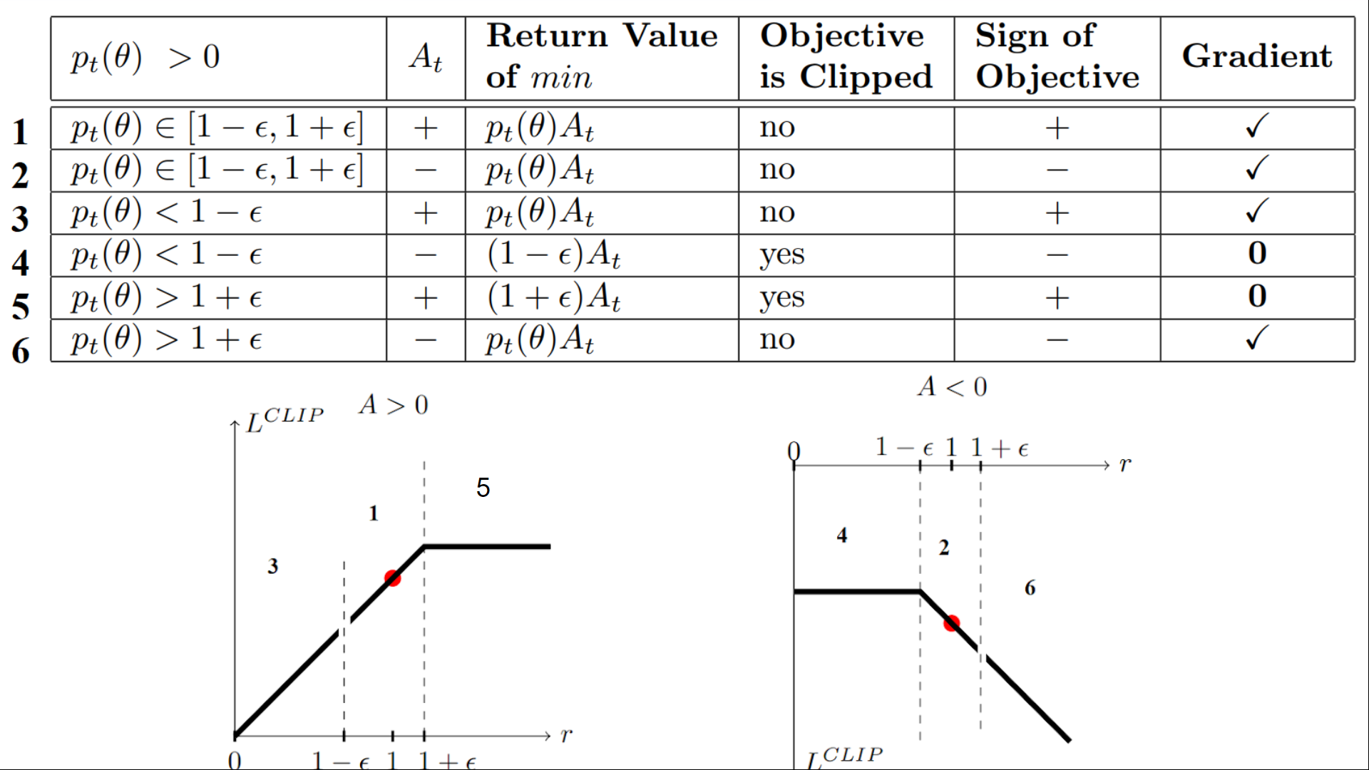
Table from “Towards Delivering a Coherent Self-Contained
Explanation of Proximal Policy Optimization” by Daniel Bick
We have six different situations. Remember first that we take the minimum between the clipped and unclipped objectives.

PPO表来自Daniel Bick所著的《为最近的政策优化提供一个连贯的、自包含的解释》我们有六种不同的情况。首先要记住的是，我们在有限制的目标和未限制的目标之间取最少的值。

Case 1 and 2: the ratio is between the range

情况1和2：比率介于

In situations 1 and 2, the clipping does not apply since the ratio is between the range [1−ϵ,1+ϵ] [1 - \epsilon, 1 + \epsilon] [1−ϵ,1+ϵ]

在情况1和2中，剪裁不适用，因为比率介于范围[1−ϵ，1+ϵ][1-\epsilon，1+\epsilon][1 epsilon，1+ϵ]之间

In situation 1, we have a positive advantage: the action is better than the average of all the actions in that state. Therefore, we should encourage our current policy to increase the probability of taking that action in that state.

在情况1中，我们有一个积极的优势：动作比该状态下所有动作的平均值更好。因此，我们应该鼓励我们目前的政策增加在那个州采取这一行动的可能性。

Since the ratio is between intervals, we can increase our policy’s probability of taking that action at that state.

由于比率介于区间之间，因此我们可以增加保单在该状态下采取该操作的概率。

In situation 2, we have a negative advantage: the action is worse than the average of all actions at that state. Therefore, we should discourage our current policy from taking that action in that state.

在情况2中，我们有一个负面优势：动作比该状态下所有动作的平均值更差。因此，我们应该阻止我们目前的政策在那种情况下采取这种行动。

Since the ratio is between intervals, we can decrease the probability that our policy takes that action at that state.

由于比率介于间隔之间，因此我们可以降低策略在该状态下采取该操作的概率。

Case 3 and 4: the ratio is below the range

情况3和4：比率低于范围

Table from “Towards Delivering a Coherent Self-Contained
Explanation of Proximal Policy Optimization” by Daniel Bick
If the probability ratio is lower than [1−ϵ] [1 - \epsilon] [1−ϵ], the probability of taking that action at that state is much lower than with the old policy.

如果概率比低于[1−−ϵ][1-\epsilon][1ϵ]，则在该状态下采取该操作的概率比旧策略的概率要低得多。

If, like in situation 3, the advantage estimate is positive (A>0), then you want to increase the probability of taking that action at that state.

如果像在情况3中一样，优势估计为正(A>0)，那么您想要增加在该状态下采取该操作的概率。

But if, like situation 4, the advantage estimate is negative, we don’t want to decrease further the probability of taking that action at that state. Therefore, the gradient is = 0 (since we’re on a flat line), so we don’t update our weights.

但是，如果像情况4一样，优势估计为负，我们不想进一步降低在该状态下采取该操作的概率。因此，梯度为=0(因为我们在一条平坦的线上)，所以我们不更新权重。

Case 5 and 6: the ratio is above the range

案例5和案例6：比率高于范围

Table from “Towards Delivering a Coherent Self-Contained
Explanation of Proximal Policy Optimization” by Daniel Bick
If the probability ratio is higher than [1+ϵ] [1 + \epsilon] [1+ϵ], the probability of taking that action at that state in the current policy is much higher than in the former policy.

如果概率比高于[1+ϵ][1+\epsilon][1+ϵ]，则当前策略中在该状态下采取该操作的概率远高于前一策略中的概率。

If, like in situation 5, the advantage is positive, we don’t want to get too greedy. We already have a higher probability of taking that action at that state than the former policy. Therefore, the gradient is = 0 (since we’re on a flat line), so we don’t update our weights.

如果像情况5一样，优势是积极的，我们不想变得太贪婪。与之前的政策相比，我们已经有更高的可能性在那个州采取这一行动。因此，梯度为=0(因为我们在一条平坦的线上)，所以我们不更新权重。

If, like in situation 6, the advantage is negative, we want to decrease the probability of taking that action at that state.

如果像在情况6中一样，优势是负面的，我们希望降低在该状态下采取该操作的概率。

So if we recap, we only update the policy with the unclipped objective part. When the minimum is the clipped objective part, we don’t update our policy weights since the gradient will equal 0.

因此，如果我们回顾一下，我们只会用未删减的客观部分来更新政策。当最小值是被剪裁的目标部分时，我们不会更新我们的策略权重，因为梯度将等于0。

So we update our policy only if:

因此，我们只有在以下情况下才会更新我们的政策：

• Our ratio is in the range [1−ϵ,1+ϵ] [1 - \epsilon, 1 + \epsilon] [1−ϵ,1+ϵ]
• Our ratio is outside the range, but the advantage leads to getting closer to the range
  • Being below the ratio but the advantage is > 0
  • Being above the ratio but the advantage is < 0

You might wonder why, when the minimum is the clipped ratio, the gradient is 0. When the ratio is clipped, the derivative in this case will not be the derivative of the rt(θ)∗At r_t(\theta) * A_t rt​(θ)∗At​ but the derivative of either (1−ϵ)∗At (1 - \epsilon)* A_t(1−ϵ)∗At​ or the derivative of (1+ϵ)∗At (1 + \epsilon)* A_t(1+ϵ)∗At​ which both = 0.

我们的比率在[1−−ϵ，1+ϵ][1-\epsilon，1+\epsilon][1−ϵ，1+ϵ]范围内。我们的比率在范围之外，但优势会导致更接近范围低于比率，但优势是>0高于比率，但优势是<0您可能想知道，当最小值是剪裁比率时，梯度是0。当削减比率时，这种情况下的导数将不是RT(∗)at r_t(\θ)*A_t RT∗(∗)at​的导数，而是(1−∗)at(1-\−)*A_t(1ϵ)​的导数或(1+ϵ)∗at(1+\epsilon)*A_t(1+ϵ)ϵatϵ的导数，两者都=0。

To summarize, thanks to this clipped surrogate objective, we restrict the range that the current policy can vary from the old one. Because we remove the incentive for the probability ratio to move outside of the interval since, the clip have the effect to gradient. If the ratio is > 1+ϵ 1 + \epsilon 1+ϵ or < 1−ϵ 1 - \epsilon 1−ϵ the gradient will be equal to 0.

总而言之，由于这个被削减的代理目标，我们限制了当前政策可以与旧政策不同的范围。因为我们去掉了概率比移动到区间之外的诱因，所以片段具有渐变的效果。如果比率大于1+−1+\epsilon 1+−或<1ϵ1-\epsilon 1ϵ，则梯度将等于0。

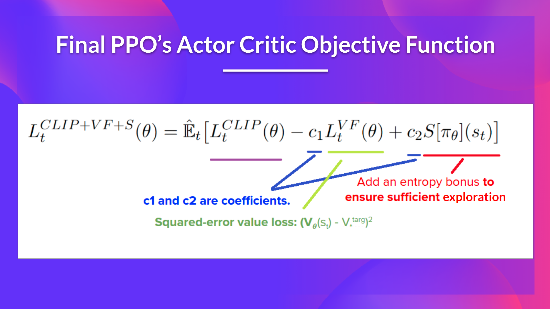
The final Clipped Surrogate Objective Loss for PPO Actor-Critic style looks like this, it’s a combination of Clipped Surrogate Objective function, Value Loss Function and Entropy bonus:

PPO演员-批评家风格的最终裁剪代理目标损失如下，它是裁剪的代理目标函数、价值损失函数和熵奖金的组合：

That was quite complex. Take time to understand these situations by looking at the table and the graph. You must understand why this makes sense. If you want to go deeper, the best resource is the article Towards Delivering a Coherent Self-Contained Explanation of Proximal Policy Optimization” by Daniel Bick, especially part 3.4.

PPO目标相当复杂。花点时间通过查看表格和图表来理解这些情况。你必须理解为什么这是有意义的。如果您想深入了解，最好的参考资料是Daniel Bick撰写的文章《为近端策略优化提供连贯而完整的解释》，尤其是第3.4部分。