E4-Unit_2-Introduction_to_Q_Learning-E4-Monte_Carlo_vs_Temporal_Difference_Learning

中英文对照学习，效果更佳！
原课程链接：https://huggingface.co/deep-rl-course/unit5/snowball-target?fw=pt

Monte Carlo vs Temporal Difference Learning

蒙特卡罗与时差学习

The last thing we need to discuss before diving into Q-Learning is the two learning strategies.

在深入Q-Learning之前，我们需要讨论的最后一件事是两种学习策略。

Remember that an RL agent learns by interacting with its environment. The idea is that given the experience and the received reward, the agent will update its value function or policy.

记住，RL代理通过与其环境互动来学习。其想法是，在给定经验和收到的奖励后，代理将更新其价值功能或策略。

Monte Carlo and Temporal Difference Learning are two different strategies on how to train our value function or our policy function. Both of them use experience to solve the RL problem.

蒙特卡罗和时差学习是关于如何训练我们的价值函数或我们的政策函数的两种不同的学习策略，它们都可以用经验来解决RL问题。

On one hand, Monte Carlo uses an entire episode of experience before learning. On the other hand, Temporal Difference uses only a step ( St,At,Rt+1,St+1S_t, A_t, R_{t+1}, S_{t+1}St​,At​,Rt+1​,St+1​ ) to learn.

一方面，蒙特卡罗在学习前使用了一整集的经验；另一方面，时差只使用了一个步骤(ST，at，RT+1，ST+1s_t，A_t，R_{t+1}，S_{t+1}St​，at​，RT+1​，ST+1​)来学习。

We’ll explain both of them using a value-based method example.

我们将使用基于值的方法示例来解释这两种方法。

Monte Carlo: learning at the end of the episode

蒙特卡洛：在这一集的结尾学习

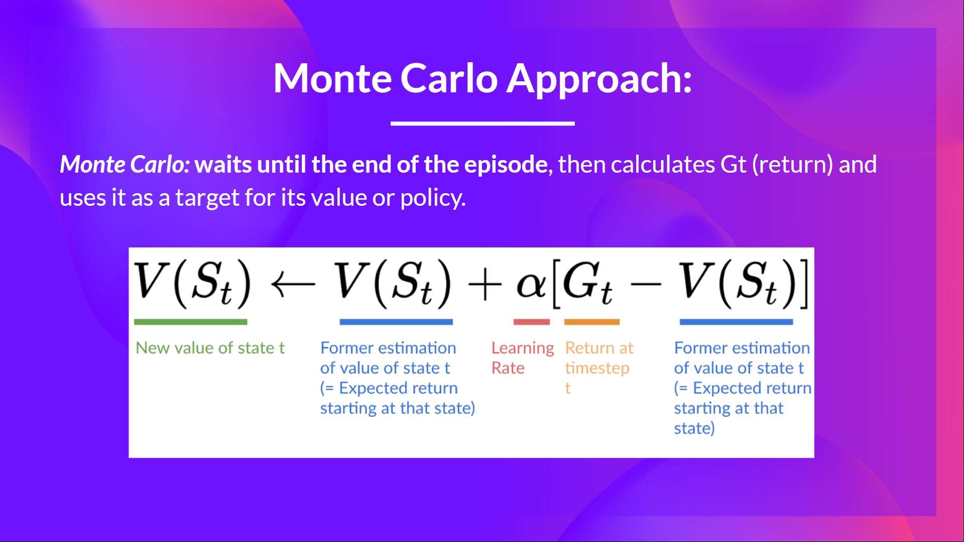
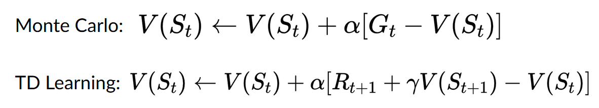
Monte Carlo waits until the end of the episode, calculates GtG_tGt​ (return) and uses it as a target for updating V(St)V(S_t)V(St​).

蒙特卡洛等到这一集结束，计算gtg_tgt​(Return)，并将其作为更新V(ST)V(S_T)V(ST​)的目标。

So it requires a complete episode of interaction before updating our value function.

因此，在更新我们的价值功能之前，需要一个完整的互动插曲。

If we take an example:

蒙特卡洛如果我们举个例子：

蒙特卡洛

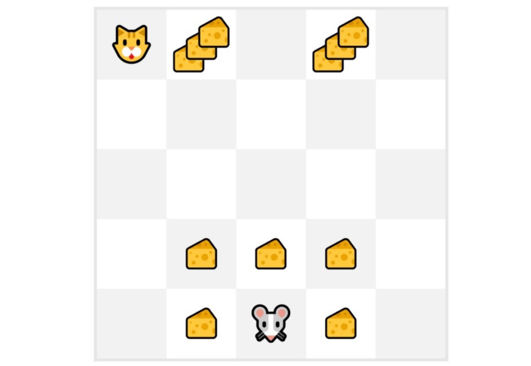
• We always start the episode at the same starting point.
• The agent takes actions using the policy. For instance, using an Epsilon Greedy Strategy, a policy that alternates between exploration (random actions) and exploitation.
• We get the reward and the next state.
• We terminate the episode if the cat eats the mouse or if the mouse moves > 10 steps.
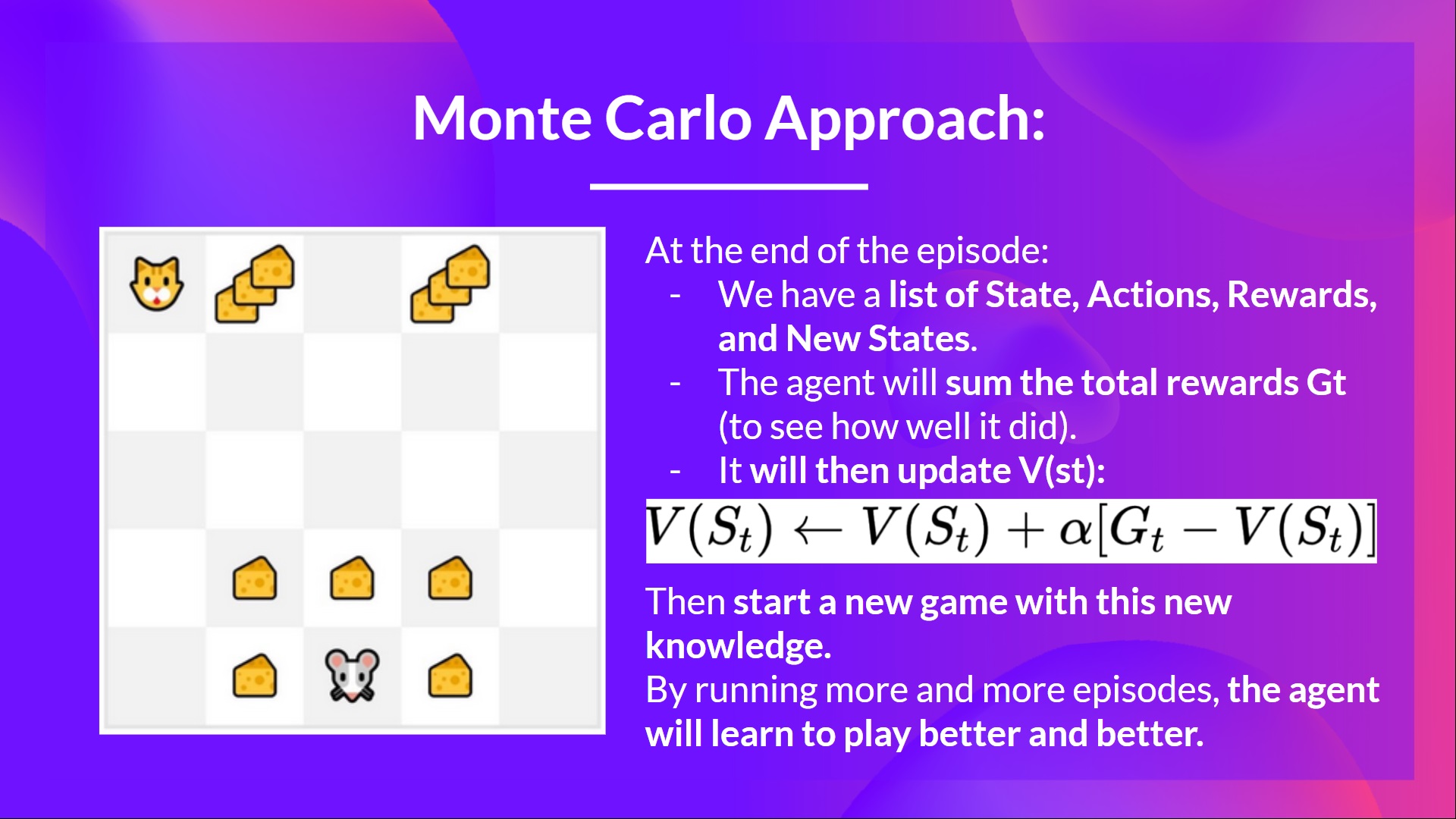
• At the end of the episode, we have a list of State, Actions, Rewards, and Next States tuples
  For instance [[State tile 3 bottom, Go Left, +1, State tile 2 bottom], [State tile 2 bottom, Go Left, +0, State tile 1 bottom]…]
• The agent will sum the total rewards GtG_tGt​ (to see how well it did).
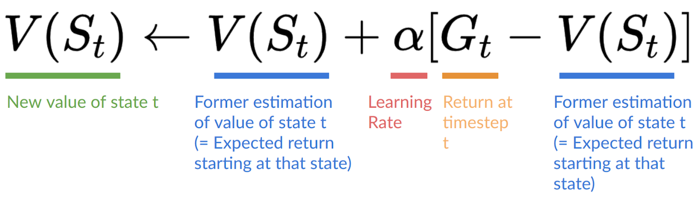
• It will then update V(st)V(s_t)V(st​) based on the formula

我们总是在同一个起始点开始这一集。代理使用策略采取行动。例如，使用Epsilon贪婪策略，这是一种在探索(随机动作)和剥削之间交替的策略。我们得到奖励和下一状态。如果猫吃了老鼠或如果鼠标移动超过10步，我们就终止这一集。在这一集的结尾，我们有一个状态、动作、奖励和下一状态元组的列表，例如[[状态块3底部，左转，+1，状态块2底部]，[状态块2底部，左转，+0，状态块1底部]…]代理将对总奖励gtg_tgt​进行求和(以查看其表现如何)。然后将基于公式蒙特卡罗更新V(St)V(S_T)V(st​

• Then start a new game with this new knowledge

By running more and more episodes, the agent will learn to play better and better.

然后用这些新知识开始一场新的游戏通过播放越来越多的剧集，经纪人会学习打得越来越好。

For instance, if we train a state-value function using Monte Carlo:

例如，如果我们使用蒙特卡罗训练状态值函数：

• We just started to train our value function, so it returns 0 value for each state
• Our learning rate (lr) is 0.1 and our discount rate is 1 (= no discount)
• Our mouse explores the environment and takes random actions

我们刚刚开始训练我们的值函数，所以它为每个状态返回0值我们的学习率(LR)是0.1，我们的贴现率是1(=没有折扣)我们的鼠标可以探索环境并采取随机操作蒙特卡洛

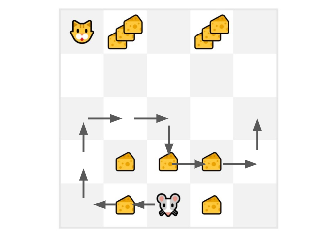
• The mouse made more than 10 steps, so the episode ends .

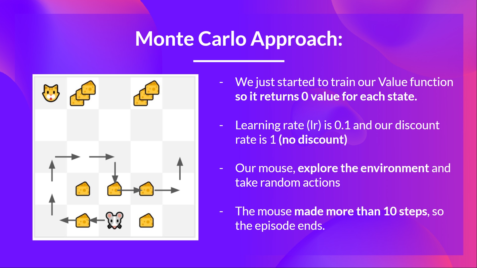
老鼠走了10多步，这一集就结束了。蒙特卡洛

• We have a list of state, action, rewards, next_state, we need to calculate the return GtG{t}Gt
• Gt=Rt+1+Rt+2+Rt+3…G_t = R_{t+1} + R_{t+2} + R_{t+3} …Gt​=Rt+1​+Rt+2​+Rt+3​…
• Gt=Rt+1+Rt+2+Rt+3…G_t = R_{t+1} + R_{t+2} + R_{t+3}…Gt​=Rt+1​+Rt+2​+Rt+3​… (for simplicity we don’t discount the rewards).
• Gt=1+0+0+0+0+0+1+1+0+0G_t = 1 + 0 + 0 + 0+ 0 + 0 + 1 + 1 + 0 + 0Gt​=1+0+0+0+0+0+1+1+0+0
• Gt=3G_t= 3Gt​=3
• We can now update V(S0)V(S_0)V(S0​):

我们有一个状态、动作、奖励、NEXT_STATE的列表，我们需要计算Gtg{t}GtGt=RT+1+RT+2+RT+3…G_t=R_{t+1}+R_{t+2}+R_{t+3}…gt​=RT+1​+RT+2​+RT+3​…gt=RT+1+RT+2+RT+3…G_t=R_{t+1}+R_{t+2}+R_{t+3}…GT​=RT+1​+RT+2​+RT+3​…(为了简单起见，我们不会打折扣)。Gt=1+0+0+0+0+1+1+0+0g_t=1+0+0+0+0+0+1+1+0+0+0+0​=1+0+0+0+0+0+1+1+0+0Gt=3G_t=3Gt​=3我们现在可以更新V(S0)V(S_0)V(S0​)：蒙特卡洛

• New V(S0)=V(S0)+lr∗[Gt—V(S0)]V(S_0) = V(S_0) + lr * [G_t — V(S_0)]V(S0​)=V(S0​)+lr∗[Gt​—V(S0​)]
• New V(S0)=0+0.1∗[3–0]V(S_0) = 0 + 0.1 * [3 – 0]V(S0​)=0+0.1∗[3–0]
• New V(S0)=0.3V(S_0) = 0.3V(S0​)=0.3

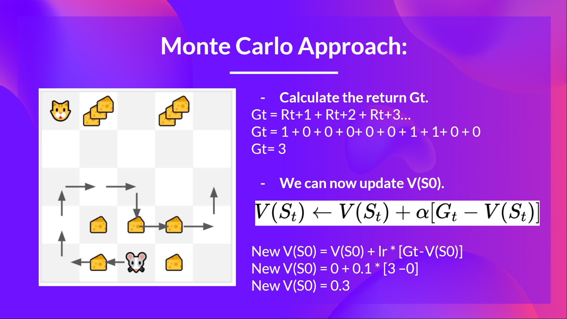
新V(S0)=V(S0)+LR∗[GT-V(S0)]V(S_0)=V(S_0)+LR*[G_t-V(S_0)]V(S0​)=V(S0​)+LR∗[GT​-V(S0​)]新V(S0)=0+0.1∗[3-0]V(S_0)=0+0.1*[3-0]V(S0​)=0+0.1∗[3-0]新V(S0)=0.3V(S_0)=0.3V(S0​)=0.3蒙特卡罗

Temporal Difference Learning: learning at each step

时差学习：每一步的学习

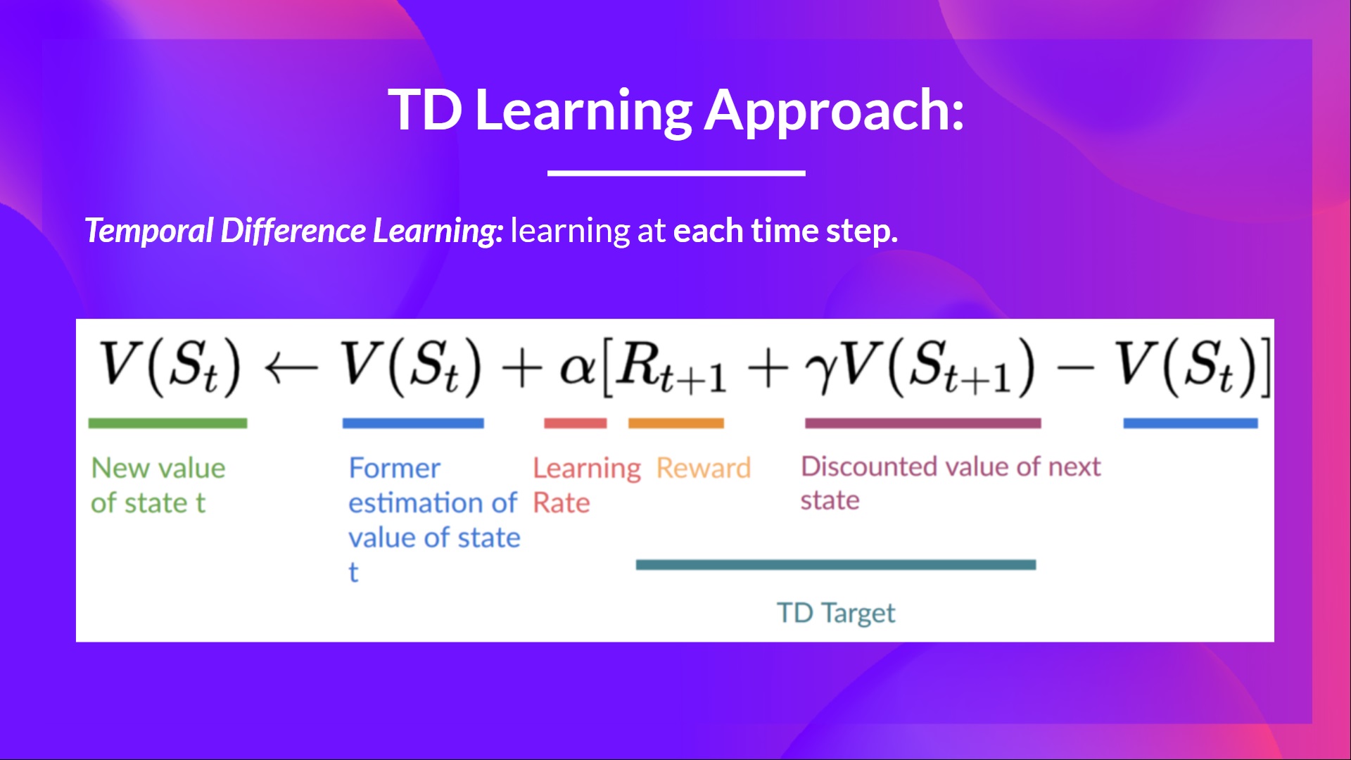
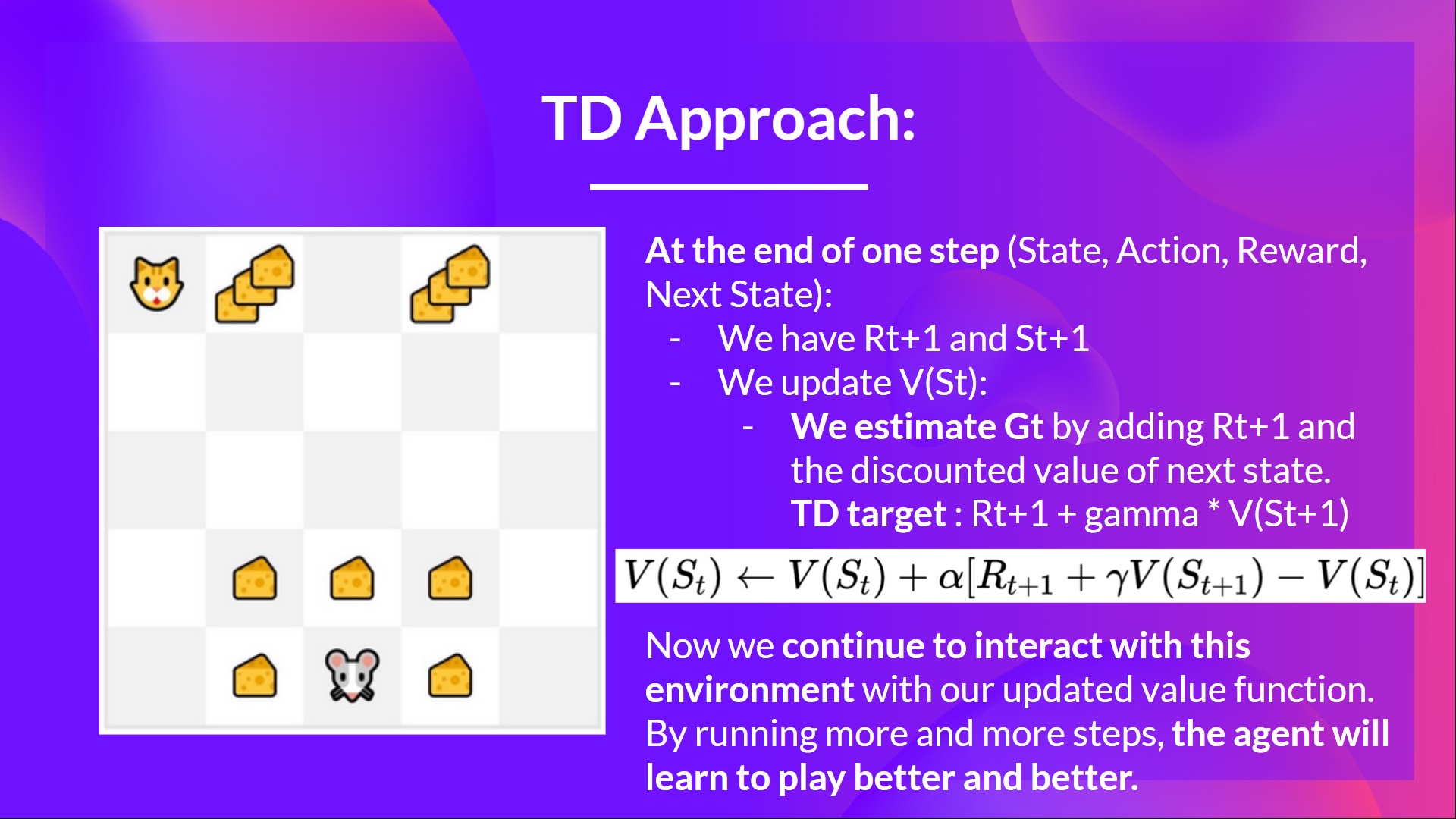
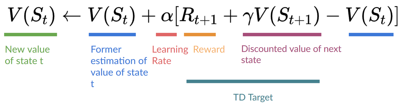
Temporal Difference, on the other hand, waits for only one interaction (one step) St+1S_{t+1}St+1​ to form a TD target and update V(St)V(S_t)V(St​) using Rt+1R_{t+1}Rt+1​ and γ∗V(St+1) \gamma * V(S_{t+1})γ∗V(St+1​).

另一方面，时差只等待一个相互作用(一步)ST+1s_{t+1}ST+1​形成TD目标，并使用RT+1R_{t+1}RT+1​和​∗V(ST+1)\∗*V(S_{t+1})​γV(ST+1γ)更新V(ST)V(S_T)V(ST_T)V(ST+1)。

The idea with TD is to update the V(St)V(S_t)V(St​) at each step.

TD的想法是在每一步更新V(ST)V(S_T)V(ST​)。

But because we didn’t experience an entire episode, we don’t have GtG_tGt​ (expected return). Instead, we estimate GtG_tGt​ by adding Rt+1R_{t+1}Rt+1​ and the discounted value of the next state.

但因为我们没有经历一整集，所以我们没有gtg_tgt​(预期收益)。相反，我们通过将rt+1rt+1 rt+1​和下一状态的折扣值相加来估计gtg_tgt​。

This is called bootstrapping. It’s called this because TD bases its update part on an existing estimate V(St+1)V(S_{t+1})V(St+1​) and not a complete sample GtG_tGt​.

这称为自举。之所以这样说，是因为TD将其更新部分基于现有的估计V(ST+1)V(S_{t+1})V(ST+1​)，而不是完整的样本GTG_TGT​。

This method is called TD(0) or one-step TD (update the value function after any individual step).

这种方法被称为TD(0)或一步TD(在任何单个步骤之后更新值函数)。

If we take the same example,

时间差如果我们举同样的例子，

时间差分

• We just started to train our value function, so it returns 0 value for each state.
• Our learning rate (lr) is 0.1, and our discount rate is 1 (no discount).
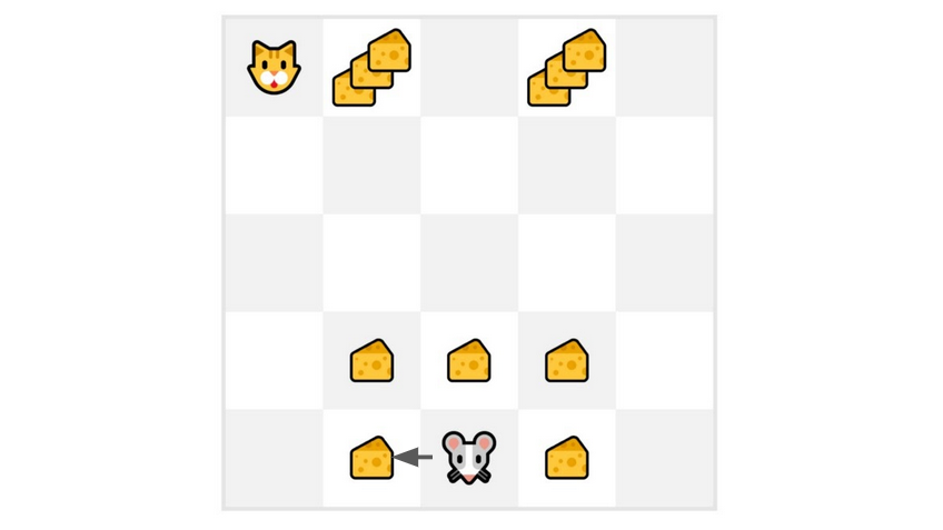
• Our mouse explore the environment and take a random action: going to the left
• It gets a reward Rt+1=1R_{t+1} = 1Rt+1​=1 since it eats a piece of cheese

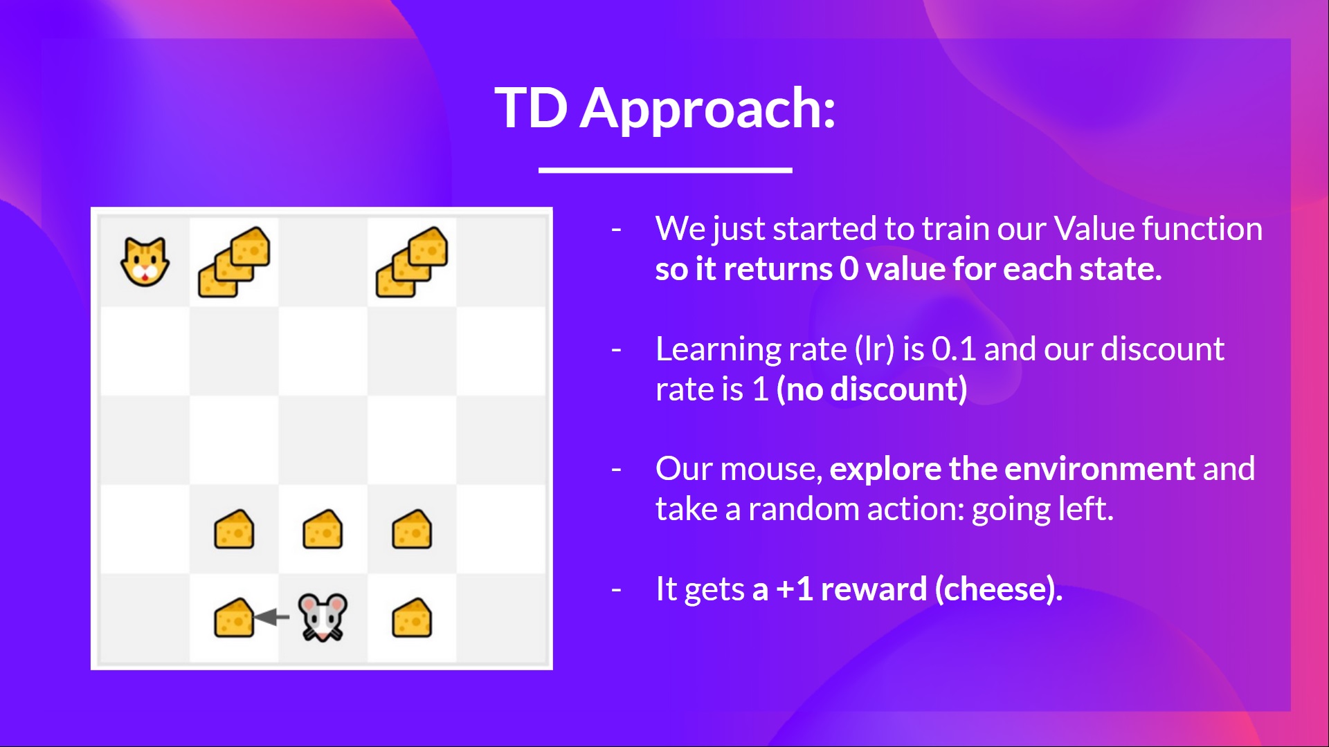
我们刚刚开始训练我们的值函数，所以它为每个州返回0值。我们的学习率(LR)是0.1，我们的贴现率是1(没有折扣)。我们的鼠标探索环境并采取随机行动：向左转它得到奖励RT+1=1R_{t+1}=1RT+1​=1，因为它吃了一块奶酪暂时的差异

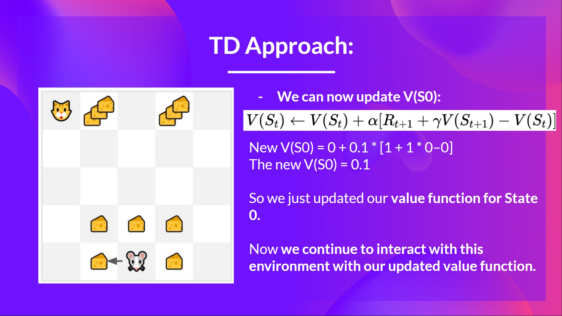
We can now update V(S0)V(S_0)V(S0​):

时间差我们现在可以更新V(S0)V(S_0)V(S0​)：

New V(S0)=V(S0)+lr∗[R1+γ∗V(S1)−V(S0)]V(S_0) = V(S_0) + lr * [R_1 + \gamma * V(S_1) - V(S_0)]V(S0​)=V(S0​)+lr∗[R1​+γ∗V(S1​)−V(S0​)]

新V(S0)=V(S0)+LR∗[R1+∗V(S1)−V(S0)]V(S_0)=V(S_0)+LR*[R_1+\γ*V(S_1)-V(S_0)]V(S0​)=V(S0∗)+LR​+∗V(S1​)−V(S0​)]

New V(S0)=0+0.1∗[1+1∗0–0]V(S_0) = 0 + 0.1 * [1 + 1 * 0–0]V(S0​)=0+0.1∗[1+1∗0–0]

新V(S0)=0+0.1∗[1+1∗0-0]V(S_0)=0+0.1*[1+1*0-0]V(S0​)=0+0.1∗[1+1∗0-0]

New V(S0)=0.1V(S_0) = 0.1V(S0​)=0.1

新V(S0)=0.1V(S_0)=0.1V(S0​)=0.1

So we just updated our value function for State 0.

因此，我们刚刚更新了状态0的值函数。

Now we continue to interact with this environment with our updated value function.

现在我们可以继续用我们更新的价值功能与这个环境互动。

If we summarize:

如果我们总结一下时间上的差异：

• With Monte Carlo, we update the value function from a complete episode, and so we use the actual accurate discounted return of this episode.
• With TD Learning, we update the value function from a step, so we replace GtG_tGt​ that we don’t have with an estimated return called TD target.

在蒙特卡洛方法中，我们根据一个完整的剧集更新值函数，因此我们可以使用这一集的实际准确贴现收益。在TD学习中，我们从一个步骤更新值函数，因此我们用一个称为TD目标的估计收益来替换我们没有的gtg_tgt​。摘要